
Abstract
This blog post is set out to build a predictive model that looks into web traffic by focusing on user sessions in a dataset taken from an e-commerce platform we shall call “GlobalGoods” for the sake of illustration. By analyzing the actions performed in website sessions and identifying key patterns that influence conversion rates, consumer behaviour can be predicted with a degree of confidence that enables the company to take corrective and proactive actions to achieve its goal, which is to drive more sales. The objective of this article is to go through the creation of that predictive model ensuring that each step of the process is reproducible and applicable to both current and future data.
Introduction
Selling products in an ever growing market of competing e-commerce platforms has become increasingly difficult. It’s essential to explore and utilize the best methods of appealing to consumers. One way to do that is to track and analyze the behaviour of customers in the e-commerce platform in question “GlobalGoods”, create appropriate prediction models, and use that as a basis to predict whether or not a customer will make a purchase.
Possessing data-driven knowledge grants the company the ability to take well informed decisions and actions. The impact of such knowledge should not be underestimated. Marketing efforts can be designed and tailored based on customer preferences, which includes personalized emails that offer products centered on interests of customers and generating recommendations that appeal to individual customers. Streamlining the website design and user experience also enables customers to seamlessly navigate through the platform and find their desired products. Dynamic price optimization can also be a powerful tool that achieves the highest profit margin possible given the product demand. There are many other ways predictive analysis can be instrumental in increasing revenue (Witten et al., 2017).
The blog post will go through several steps, broadly: preparing the data, performing exploratory analysis, selecting and applying the predictive models, assessing the validity of those models, and finally, drawing conclusions and recommendations. The objective is to establish and utilize a reliable predictive model that predicts whether or not a user session will result in a purchase.
Literature Review
The dataset that will be used as a basis for the analysis is “Online Shoppers Purchasing Intention Dataset” which describes the user session in the hypothetical platform “GlobalGoods”. This dataset contains quite a lot of sessions, 12,330 to be exact. It is worth noting that the vast majority, 84.5% (meaning 10,422) of those sessions, did not actually lead to a sale. On the other hand, the smaller slice, 15.5% or 1,908 sessions, did end with shoppers making a purchase. (C. Sakar, 2018)
The structure of the dataset is optimum for the kind of analysis that will be conducted here. Each session is packed with details, creating a rich summary of user activity. Every single session is linked to a unique user, stretched out over a whole year. The data was formed in a way that avoids any skew towards particular promos, holidays, user types, or specific times, so it gives a well-rounded view, free from the usual biases.
This blog post looks into the “Online Shoppers Purchasing Intention Dataset” to find out what makes customers at “GlobalGoods” decide to buy or not. Analysis techniques like Logistic Regression will be utilized as it performs well in predicting user activity based on browsing history. Also, Random Forest will be used for its ability to accurately process complex datasets, and others. Finding out what makes a shopping session end in a purchase is key here.
In the development of the desired system of analysis throughout the article, Python programming language will be utilized. Python is easy to use and set up, and it allows the system to be tweaked, reproduced and/or applied on future data. Focus will be placed on readability and comprehensiveness.
Discussion and Analysis
This section represents the essence of this exercise as it will go over the steps of the development of the prediction model, starting with preparing the dataset. For the sake of brevity, the dataframe name in the Python programming environment is df. This dataset of 12,330 rows contains a multitude of features reflecting details regarding user activity within each user session.
Data and Environment Preparation
First of all, we’ll start with loading all the libraries at once:
					import pandas as pd
import os
import re
import numpy as np
import requests
import matplotlib.pyplot as plt
from datetime import datetime
from io import StringIO
import seaborn as sns
from sklearn.cluster import KMeans
from sklearn.decomposition import PCA
from sklearn.preprocessing import StandardScaler, OneHotEncoder
from sklearn.compose import ColumnTransformer
from sklearn.pipeline import make_pipeline
from sklearn.ensemble import RandomForestClassifier
from sklearn.metrics import classification_report, confusion_matrix, accuracy_score
from sklearn.model_selection import train_test_split
from sklearn.linear_model import LogisticRegression
from sklearn.metrics import RocCurveDisplay
from sklearn.ensemble import GradientBoostingClassifier
The Month column contains 3 letter month names, except for June which has 4 letters. It would be wise to convert the column to numeric categories, like so:
					# Replace 'June' with 'Jun' in the 'Month' column
df['Month'] = df['Month'].replace('June', 'Jun')

# Convert 'Month' abbreviations to month numbers and store in a new column 'Month_No'
df['Month_No'] = df['Month'].apply(lambda x: datetime.strptime(x, '%b').month)

df = df.drop('Month', axis=1)
To streamline the analysis of the dataset in the coming steps, the columns have been categorized into column groups: categorical, integer, float, and percentage columns, ensuring that the column types are explicitly defined and enforced. Doing that will accurately preserve the essence of these variables within the analyses.
					# Manually define lists of columns for each type
categorical_columns = ['Month_No', 'OperatingSystems', 'Browser', 'Region', 'TrafficType', 'VisitorType', 'Weekend', 'Revenue']
integer_columns = ['Administrative', 'Informational', 'ProductRelated']
percentage_columns = ['BounceRates', 'ExitRates', 'SpecialDay']  # Columns with values between 0 and 1
float_columns = ['Administrative_Duration', 'Informational_Duration', 'ProductRelated_Duration', 'PageValues']

# Combine integer, percentage, and other float columns for a full list of numeric columns
float_and_integer_columns = integer_columns + float_columns
numeric_columns = integer_columns + percentage_columns + float_columns

# Convert categorical columns to 'category' type
for column in categorical_columns:
    df[column] = df[column].astype('category')

# Convert integer columns to 'int' type, handling NaN values with 'Int64' type
for column in integer_columns:
    df[column] = pd.to_numeric(df[column], errors='coerce').astype('Int64')

# Convert percentage columns to 'float' type, ensuring they remain between 0 and 1
for column in percentage_columns:
    df[column] = pd.to_numeric(df[column], errors='coerce').astype('float')

# Convert other float columns to 'float' type
for column in float_columns:
    df[column] = pd.to_numeric(df[column], errors='coerce').astype('float')
Categorical columns, which are the predominant data type in the dataset, include: Month_No, OperatingSystems, Browser, Region, TrafficType, VisitorType, as well as binary variables such as Weekend and Revenue. On the other hand, the dataset contains numeric columns: Administrative, Informational, ProductRelated, alongside their corresponding durations. And lastly, columns that contain values between 0 and 1: BounceRates, ExitRates and SpecialDay also have their own category. It is worth noting that this dataset does not contain missing values and therefore there is no need to create logic for that.
Exploratory Data Analysis
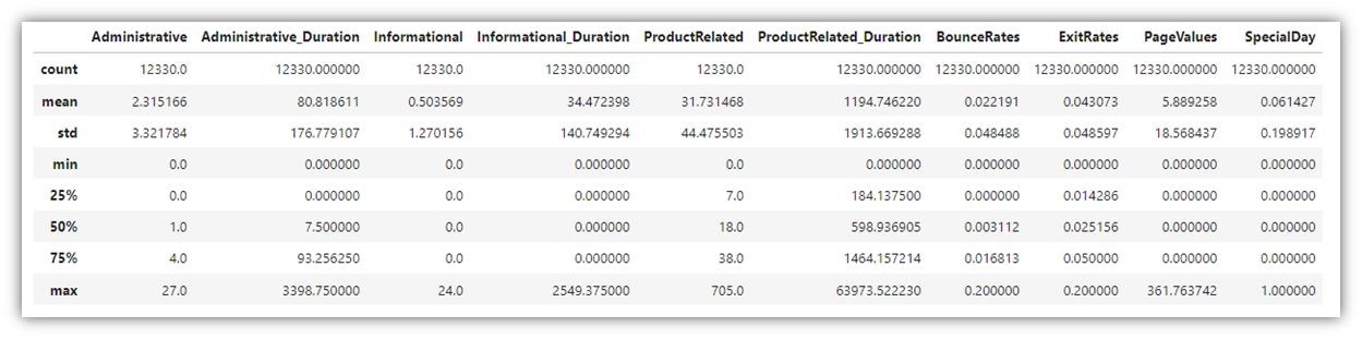
Before analyzing the data, we need to familiarize ourselves with its contents, and search for patterns and insights. Exploring the data is a crucial step where many visuals are generated in order to identify general trends in the variables, understand the relationship among different combinations of variables, and take note of outlier values that exist within the individual columns. In this case, it is important to generally recognize which factors or user activities contribute to the decision of making a purchase in the site. For that, many visuals need to be created at once in the aim of finding something that stands out. Let’s start with creating a summary table for all the numeric variables in the data frame:
df.describe()
Next, let’s explore how the column “Revenue” relates to other categorical variables. In order to go through all the visuals at once, a for loop was created:
for column in categorical_columns:
    # Adjusting the size and clarity of the plot for each categorical column
    plt.figure(figsize=(14, 8))
    ax = sns.countplot(x=column, hue='Revenue', data=df, palette=palette, hue_order=[True, False])
    plt.title(f"Distribution of {column} by Revenue", fontsize=16)
    plt.xticks(fontsize=12)
    plt.xlabel(column, fontsize=14)
    plt.ylabel('Count', fontsize=14)

    plt.tight_layout()
    plt.show()
This produces bar charts that visualize each categorical variable in relation to the Revenue column. The above code produces eight charts, the below are two examples of them:
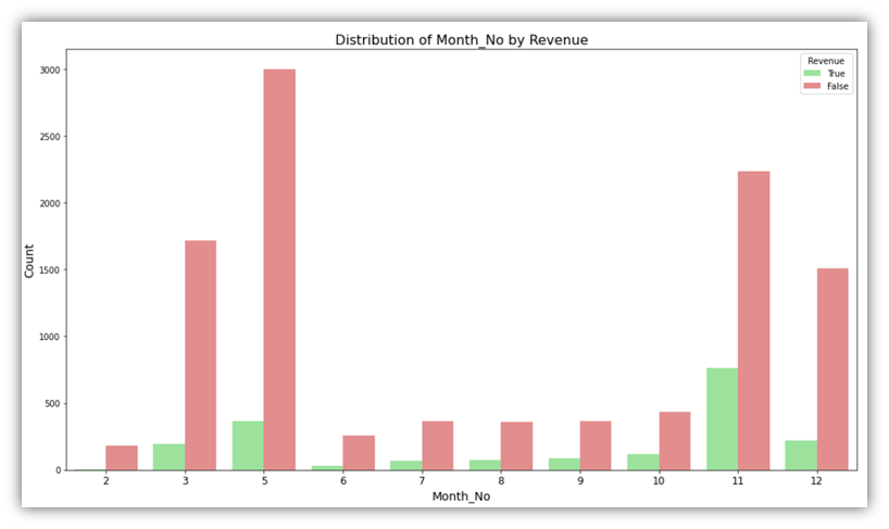
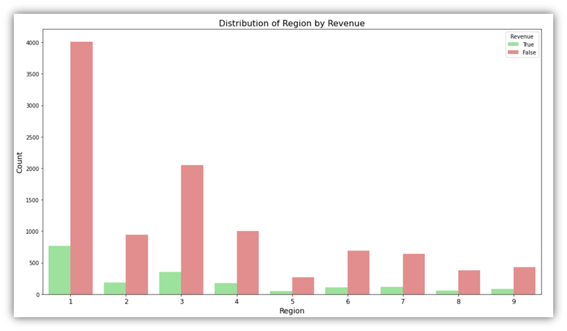
These charts describe how the Revenue column is associated with other categories like month. In the first visual, we can see that in month number 2, there has been almost no sessions that ended up with a purchase, while in month number 11, more that a third of user sessions ended up with a purchase.
Looking at the same categorical variables, we can visualize the percentages of the Revenue column with better clarity. Here is the code for creating another set of visuals that focus on the percentages of Revenue in each category:
					# Assuming df, categorical_columns, and palette are defined
for column in categorical_columns:
    x, y = column, 'Revenue'
    df1 = df.groupby(x)[y].value_counts(normalize=True)
    df1 = df1.mul(100)
    df1 = df1.rename('percent').reset_index()

    # Adjust figsize here by using the size and aspect parameters in sns.catplot()
    g = sns.catplot(x=x, y='percent', hue=y, kind='bar', data=df1,
                    palette=palette, hue_order=[True, False], height=6, aspect=2)
    g.ax.set_ylim(0, 100)

    # Ensure that the text annotation uses a float for the height and rounds correctly,
    # and skip annotating bars with a height of 0 or near 0 to avoid '0.00%' labels where they don't make sense.
    for p in g.ax.patches:
        height = p.get_height()
        if height > 0:  # Only annotate bars with a height greater than 0
            txt = f"{height:.0f}%"
            txt_x = p.get_x() + p.get_width() / 2.
            txt_y = height
            g.ax.text(txt_x, txt_y, txt, ha='center', va='bottom')

    # Improve legend appearance
    plt.legend(title='Revenue', bbox_to_anchor=(0.95, 1.05), loc=2, borderaxespad=0.)
    g._legend.remove()

    plt.tight_layout()
    plt.show()
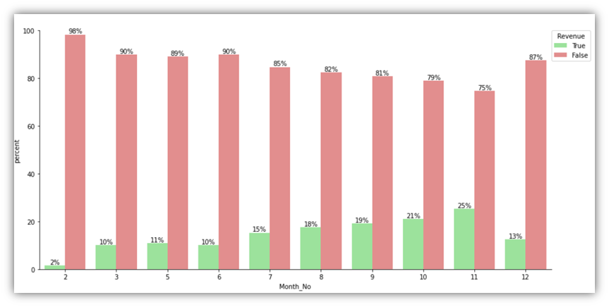
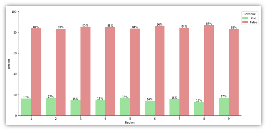
It can be noticed that the conclusions drawn from the previous charts are different from the conclusions drawn from these charts. For example, when it comes to Region, there’s obviously a variability on the traffic and number of successful sessions. However, looking at the percentages visual, it can be seen that throughout all the regions, roughly the same percentage of successful sessions occurred out of all sessions.
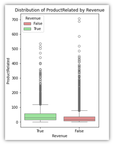
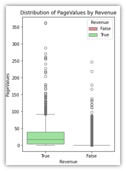
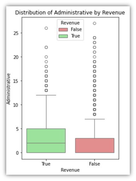
Next, let’s look at float and integer columns relative to the Revenue column:
for column in float_and_integer_columns:
    plt.figure(figsize=(4, 6))
    sns.boxplot(x=df['Revenue'], y=column, hue=df['Revenue'],
                data=df, order=[True, False], palette=palette)
    plt.title(f'Distribution of {column} by Revenue')
    plt.xlabel('Revenue')
    plt.ylabel(column)
    plt.show()
The following are three examples of the results:
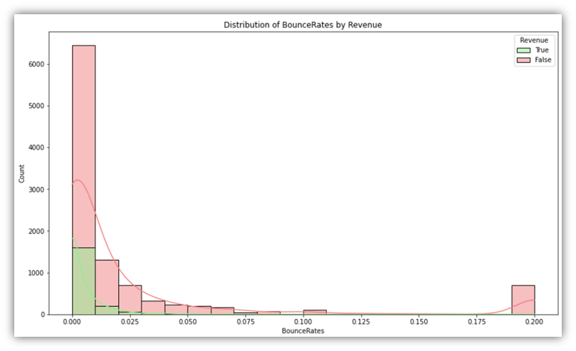
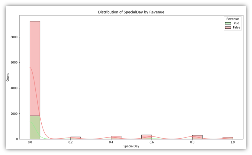
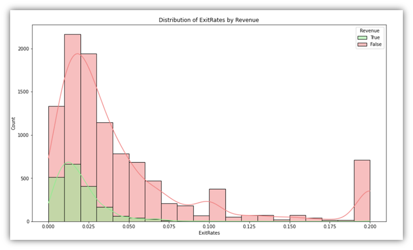
The last column group we’ll examine is the percentage group, which consists of three columns that have values ranging from 0 to 1.
for column in percentage_columns:
    plt.figure(figsize=(14, 8))
    sns.histplot(data=df, x=column, hue='Revenue', bins=20,
                 kde=True, palette=palette, hue_order=[True, False])
    plt.title(f"Distribution of {column} by Revenue")
    plt.show()
This code generates the following:
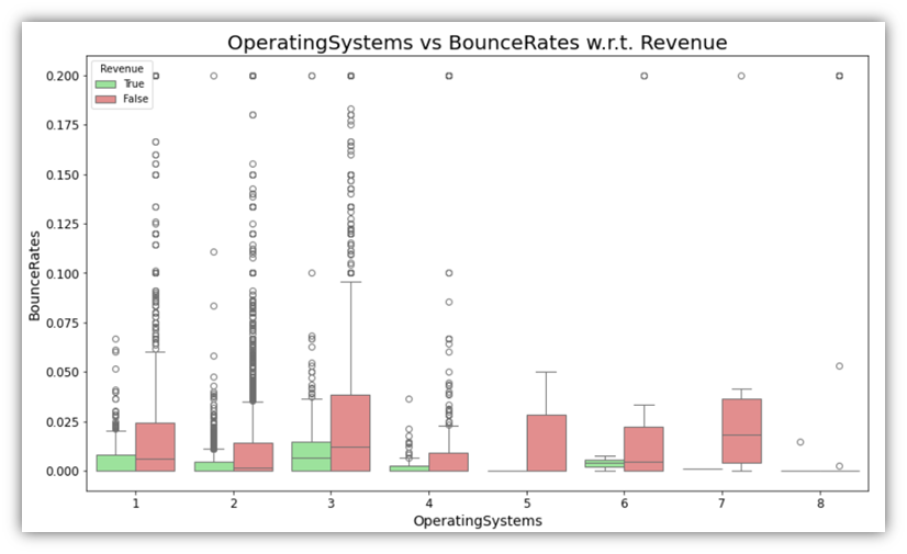
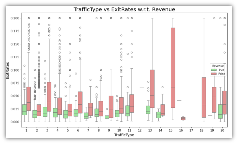
Additionally, as a way of exploring more than one variable along with the Revenue, boxplot plots can be used to provide more context to categories. It can be insightful to visualize combinations of one categorical and one numeric variable in addition the Revenue variable.
for cat_var in categorical_columns:
    for perc_var in percentage_columns:
        plt.figure(figsize=(14, 8))
        sns.boxplot(x=df[cat_var], y=df[perc_var], hue=df['Revenue'], palette=palette, hue_order=[True, False])

        plt.title(f'{cat_var} vs {perc_var} w.r.t. Revenue', fontsize=20)
        plt.xlabel(cat_var, fontsize=14)
        plt.ylabel(perc_var, fontsize=14)
        plt.xticks(fontsize=12)
        plt.yticks(fontsize=12)

        plt.show()
Examples of the results are as follows:
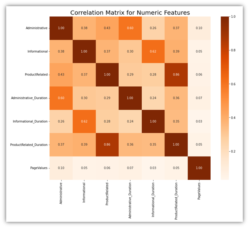
Moving to correlation analysis, let’s explore the relationships among numeric columns to identify any arising correlation pattern. There are two possible ways to do that on all numeric variables at once:
Correlation matrix is a great tool for identifying related variables among all numeric variables:
					# Calculate the correlation matrix for the combined numeric features
corr_matrix = df[numeric_columns].corr()

# Visualize the correlation matrix
plt.figure(figsize=(12, 10))
sns.heatmap(corr_matrix, annot=True, fmt=".2f", cmap='Oranges')
plt.title('Correlation Matrix for Numeric Features', fontsize=20)
plt.show()
Another method is creating a pair plot for all the numeric variables. Its similar to creating different scatterplots for different combinations of two variables:
					# Create a pair plot for a selection of combined numeric features
sns.pairplot(df.sample(500)[float_and_integer_columns], height=3, plot_kws={'alpha':0.6})
plt.suptitle('Pair Plot for Numeric Features', fontsize=20, y=1.02)
plt.show()
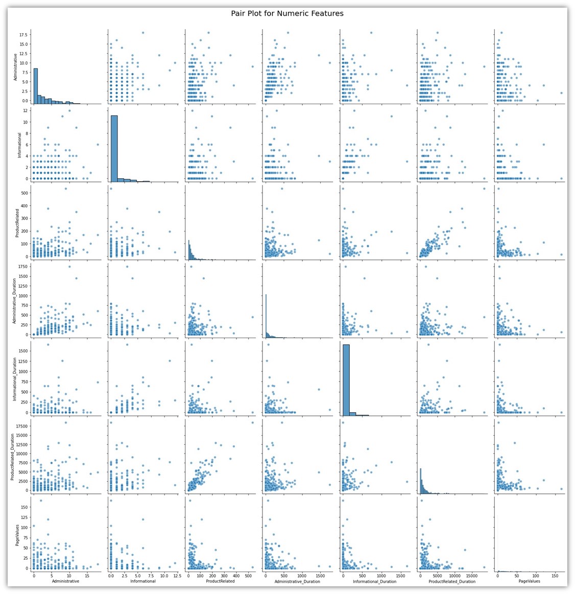
Both of these visuals show how each variable is tied to the other variable. It can be seen that only few variables show significant correlation. The correlations among those variables are natural. For example, the column ProductRelated is a column naturally tied to ProductRelated_Duration for a simple reason which is the fact that a user has to open ProductRelated pages before spending time on those pages.
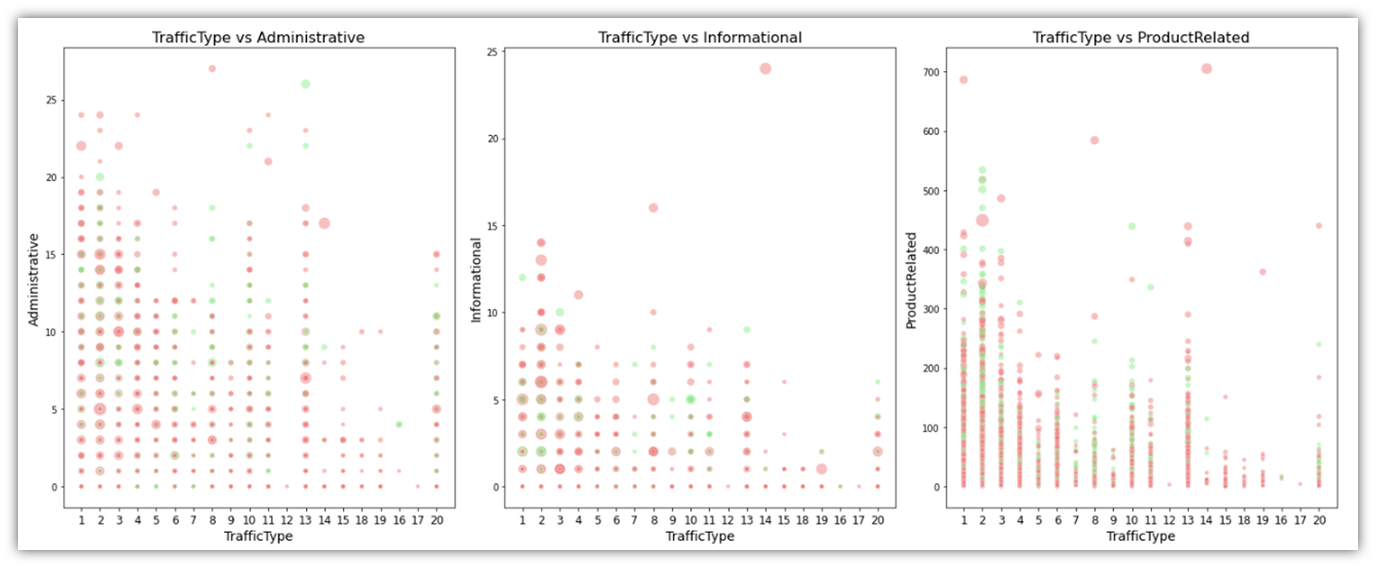
We can also look through the differences between Informational, Administrative, and ProductRelated pages and their durations categorized by TrafficType and colored by Revenue status using a scatter plot, with the durations represented as dot size.
					# Ensure TrafficType is treated as a categorical variable
df['TrafficType'] = df['TrafficType'].astype(str)

# Setting the figsize as per previous visuals
plt.figure(figsize=(20, 8))

# Lists of the variables and corresponding sizes
integer_columns = ['Administrative', 'Informational', 'ProductRelated']
duration_columns = ['Administrative_Duration', 'Informational_Duration', 'ProductRelated_Duration']

for i, column in enumerate(integer_columns):
    # Create a subplot for each combination
    plt.subplot(1, 3, i+1)  # 1 row, 3 columns, subplot index i+1

    # Creating the scatter plot
    sns.scatterplot(x='TrafficType', y=column, data=df,
                    hue='Revenue', palette=palette,
                    size=df[duration_columns[i]], alpha=0.5,
                    sizes=(20, 200), legend=False)  # Adjust dot sizes as needed

    plt.title(f'TrafficType vs {column}', fontsize=16)
    plt.xticks(fontsize=12)
    plt.xlabel('TrafficType', fontsize=14)
    plt.ylabel(column, fontsize=14)

# Adjust layout and display the combined plot
plt.tight_layout()
plt.show()
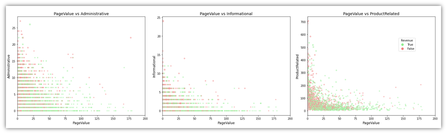
Another variable we can gain insight from is PageValue, specifically when projected in scatter plots with page types (Informational, Administrative, PageRelated) and Revenue:
					# Define the figure for the subplots
# Assuming df, page_types, durations, and palette are already defined
# Define the figure for the subplots
fig, axes = plt.subplots(1, 3, figsize=(22, 6))  # 1 row, 3 columns
page_types = ['Administrative', 'Informational', 'ProductRelated']
durations = ['Administrative_Duration', 'Informational_Duration', 'ProductRelated_Duration']

for i, (page_type, duration) in enumerate(zip(page_types, durations)):
    # Create each scatter plot with specified dot sizes
    sns.scatterplot(ax=axes[i], x='PageValues', y=page_type,
                    data=df[df['PageValues'] <= 200],  # Limit data to PageValues <= 200
                    size=df[duration] * 10,  # Adjusted for visibility
                    alpha=0.5, hue='Revenue', palette=palette, legend=False)

    # Set titles and adjust axes labels
    axes[i].set_title(f'PageValue vs {page_type}', fontsize=14)
    axes[i].set_xlabel('PageValue', fontsize=12)
    axes[i].set_ylabel(page_type, fontsize=12)
    axes[i].set_xlim([0, 200])  # Visually limit width to PageValue of 200

# Adjust layout
plt.tight_layout()

# Show the legend outside the plots
# Since legend=False in scatterplot, we manually add a legend based on 'Revenue'
# Create custom legend handles
from matplotlib.lines import Line2D
legend_handles = [Line2D([0], [0], marker='o', color='w', markerfacecolor=palette[True], markersize=10, label='True'),
                  Line2D([0], [0], marker='o', color='w', markerfacecolor=palette[False], markersize=10, label='False')]
fig.legend(handles=legend_handles, title='Revenue', bbox_to_anchor=(0.9, 0.7), loc='center left')

# Display the plot
plt.show()
This will result in the below visual:
Cluster Analysis
An integral part of our objective is to understand customer segments based on various factors within the data. This can greatly help inform the predictive model that we are constructing in addition to being a great tool for targeted marketing (Aggarwal and Reddy, 2014). With this method we can observe the behavior of various customer groups or clusters without having to explicitly tell the computer what to look for. Its like discovering organic clusters among our customers according to what they purchase how frequently they come in and what interests them. We can improve our plans for reaching out to each group make more accurate product suggestions and enhance and personalize their shopping experience by identifying these clusters. The great thing about cluster analysis is that it is flexible enough to handle a wide range of data types and can adapt as our understanding of our clients changes. We can find clever ways to boost sales on the GlobalGoods platform by using this method which is very helpful in making sense of the complicated world of online shopping.
We start by selecting the features that we want to analyze and divide into clusters. In this implementation, ‘ProductRelated’, ‘ExitRates’ were chosen. However, the code was written in a way that allows for easy replacement of variables. The features and the number of the desired clusters can easily be plugged into the code before running it. This enables quick trial and error granting the ability to identify the features that are most fit for clustering.
					# Preparing the data
features = df[['PageValues', 'Administrative', 'Informational', 'ProductRelated']]
scaler = StandardScaler()
features_scaled = scaler.fit_transform(features)

# Choosing the number of clusters (K) using the Elbow Method
inertia = []
for k in range(1, 11):
    # Explicitly setting n_init to 10
    kmeans = KMeans(n_clusters=k, random_state=42, n_init=10)
    kmeans.fit(features_scaled)
    inertia.append(kmeans.inertia_)

# Plotting the Elbow Method graph
plt.figure(figsize=(10, 6))
plt.plot(range(1, 11), inertia, marker='o')
plt.title('Elbow Method for Optimal K')
plt.xlabel('Number of clusters')
plt.ylabel('Inertia')
plt.show()
This is the resulting Elbow Method visual:
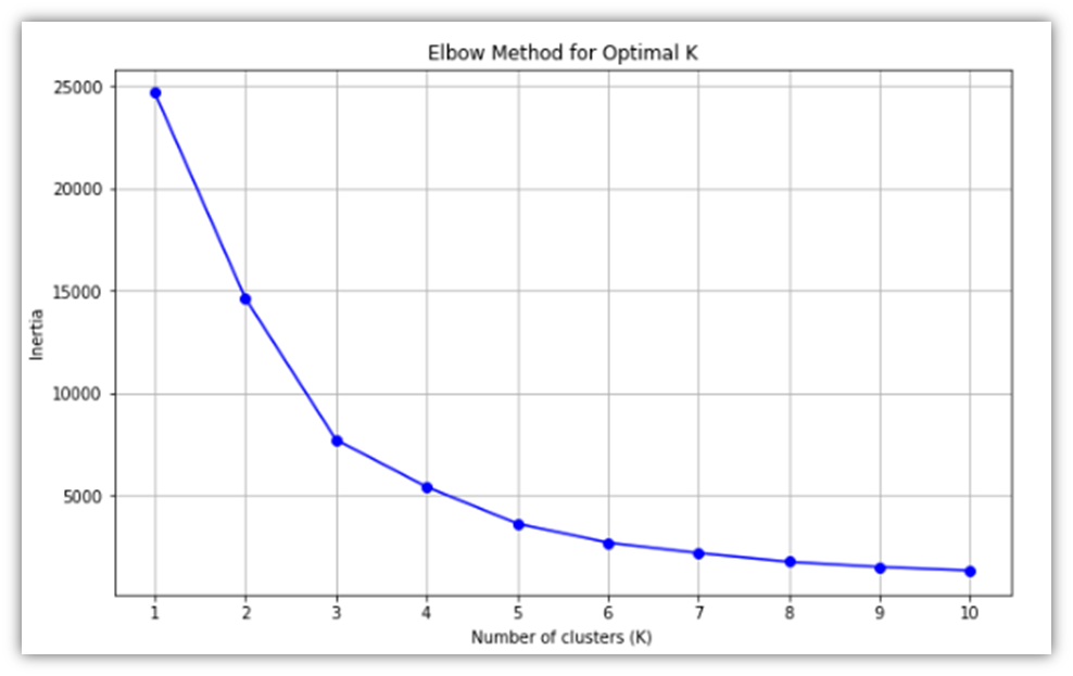
Using that visual, we can decide on the number of clusters that we will be working on. 3 or 4 clusters would be reasonable as can be seen from the line slope change. Here, 4 clusters is the cluster size of choice.
A scatter plot is a great visual for showing how the clusters are distributed within the data:
					# Perform K-means clustering with 4 clusters
kmeans = KMeans(n_clusters=cluster_size, random_state=42, n_init=10)
df['Cluster'] = kmeans.fit_predict(features_scaled)

# Scatter plot of clusters using scaled features
plt.figure(figsize=(10, 6))
sns.scatterplot(x=features_scaled[:, 0], y=features_scaled[:, 1], hue=df['Cluster'], palette='viridis', alpha=0.6, legend='full')

# Plotting centroids with marker changed to black stars
plt.scatter(kmeans.cluster_centers_[:, 0], kmeans.cluster_centers_[:, 1], s=200, c='#DD6E0F', marker='*', label='Centroids')

# Adding titles and labels with scaled notation for clarity
plt.title('Scatter Plot of Clusters with Centroids')
plt.xlabel('Scaled ' + x)
plt.ylabel('Scaled ' + y)
plt.legend(title='Cluster')
plt.show()
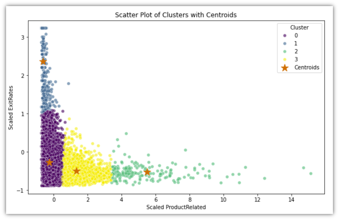
Looking at the scatter plot of the four clusters, it can guide the process of segmenting the customers. Cluster 0, for example, is the group of sessions where most users promptly exited the site without opening ProductRelated pages. Cluster 1 describes the group of sessions where most users repeatedly existed the site without going through the ProductRelated pages, indicating that they were mildly interested in the site content. Cluster 2 describes users who go through the ProductRelated pages without noticeable exit rate, so it might represent the users who would make a purchase if presented with satisfactory products. Finally, cluster 3 is the moderate combination of 1 and 2, so it would make since to target them with the intention of bringing them closer to cluster 2.
Before moving forward, let’s attempt to validate the clustering using the Revenue variable. To do that, the table is grouped by clusters along with summarized average Revenue. Here’s the code to create that table and to also visualize it in a chart:
					# Calculate the distribution of Revenue within each cluster
cluster_revenue_distribution = df.groupby('Cluster')['Revenue'].value_counts(normalize=True).unstack().fillna(0)

# Convert the distribution to a more readable percentage format
cluster_revenue_percentage = cluster_revenue_distribution * 100

print(cluster_revenue_percentage)

cluster_revenue_percentage.plot(kind='bar', stacked=True, figsize=(10, 6), color=['skyblue', 'lightgreen'])
plt.title('Revenue Distribution by Cluster')
plt.xlabel('Cluster')
plt.ylabel('Percentage')
plt.legend(title='Revenue', labels=['False', 'True'])
plt.xticks(rotation=0)
plt.grid(axis='y', linestyle='--')

plt.show()
The code will result in the following table and chart:
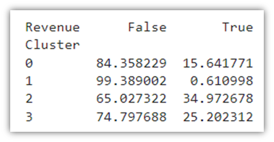
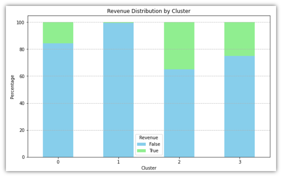
The average sessions resulting in a True value of Revenue across the entire dataset is 15.47%. Through the clustering method, we were able to divide the dataset into 4 distinct clusters where the Revenue percentages are relatively varied. Looking at Cluster 1, for example, we notice that the conversion rate is less than 1%, which would prompt further analysis into the sessions within that cluster to identify the reasons for low instances of purchase.
Exploratory data analysis makes use of a multitude of visuals to deconstruct the data packed in a large dataset. Detecting patterns and trends within the data helps inform the approaches to be taken for further analysis. We looked at different ways of slicing the data using iterative visual generation technique for pre-grouped feature columns. We looked at different metrics describing user behaviour and how they relate to each other using box plots, histograms, and scatter plots. We were also able to group the data into clusters, test for the validity of those clusters, and discuss the possible meanings of the cluster segmentation.
Predictive Analysis
Our decision on the Predictive Analysis models to be used will be based on the types of features we have. The logical first method of choice is Logistic Regression. Logistic Regression is used when attempting to predict a Boolean variable, or to put it simply, it is utilized to predict a single outcome out of two possible outcomes (Hastie, Tibshirani and Friedman, 2017). We employ logistic regression as a first choice because it is simple and efficient in our work to determine which customers will make purchases from GlobalGoods. This approach is useful for determining whether an event such as a customers purchase will occur or not. It is very effective in demonstrating to us the various factors that can influence a customer’s likelihood of making a purchase such as the frequency of their visits to our website. Because it is simple to use and comprehend, Logistic Regression greatly aids us in determining the factors that influence a customers decision to purchase. Logistic regression plays a crucial role in our research by enabling us to identify distinct trends in the online shopping habits of our customers. It can be a great predictive tool in our arsenal since our goal is to predict a binary outcome, namely, whether or not a user session will result in a purchase.
The following code is how to implement it:
					df3 = pd.get_dummies(df)
X = df3.drop(['Revenue_True', 'Revenue_False'], axis=1)
y = df['Revenue'].astype(int)  # Ensuring 'Revenue' is numeric

# Split the dataset into training and testing sets
X_train, X_test, y_train, y_test = train_test_split(X, y, test_size=0.3, random_state=42)

# Standardizing the features (important for Logistic Regression)
scaler = StandardScaler()
X_train_scaled = scaler.fit_transform(X_train)
X_test_scaled = scaler.transform(X_test)

# Logistic Regression
log_reg = LogisticRegression(max_iter=300, random_state=42)
log_reg.fit(X_train_scaled, y_train)  # Using scaled features

# Predictions
log_reg_predictions = log_reg.predict(X_test_scaled)
The above code does several steps before starting the regression. First, it one-hot encodes the dataframe using the get_dummies function which reshapes the table as to prepare it for machine learning, converting unique values in categorical variables to columns with binary values. Second, it removes the target variable that we want to predict from the dataframe and assigns it to X, and then converts binary Revenue value to integer and assigns it to y. Then it splits our dataset into two parts, one is used to train the dataset, and the other is used to test the prediction model. Next it scales the variables so that the scale of one variable does not overwhelm the other. Lastly, the Logistic Regression is performed and the data gets trained using the training set. At this point, the accuracy of model has to be tested, and for that we’ll use a confusion matrix:
					# Logistic Regression Confusion Matrix
log_reg_cm = confusion_matrix(y_test, log_reg_predictions)
sns.heatmap(log_reg_cm, annot=True, fmt='d', cmap='Purples')
plt.title('Logistic Regression Confusion Matrix')
plt.xlabel('Predicted')
plt.ylabel('True')
plt.show()
# Logistic Regression Model Accuracy
log_reg_accuracy = accuracy_score(y_test, log_reg_predictions)
print(f"\nLogistic Regression Model Accuracy: {log_reg_accuracy:.4f}")

# Logistic Regression Model Report
print("Logistic Regression Model Classification Report:")
print(classification_report(y_test, log_reg_predictions))
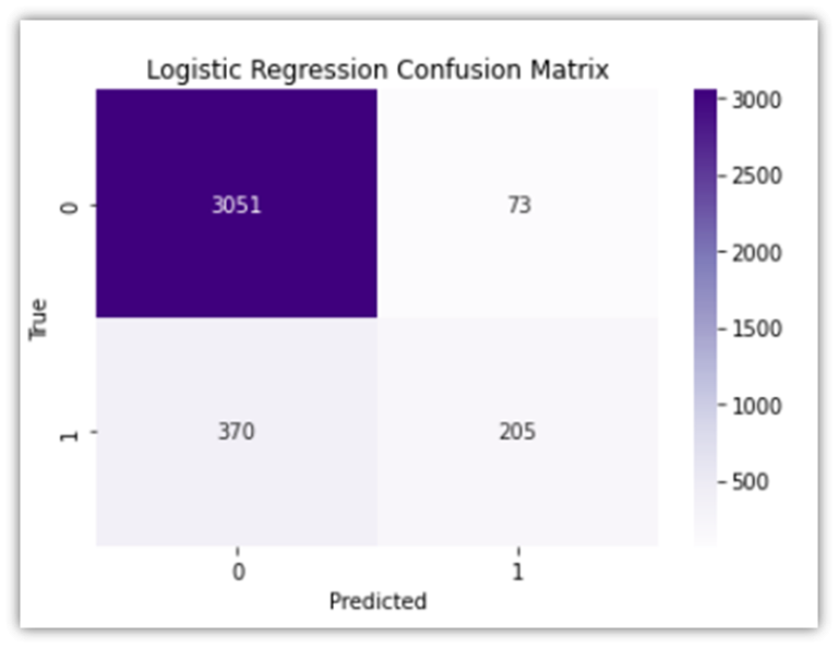
The confusion matrix above highlights the following:
• True Negative (upper left): cases where the model correctly predicts the negative class (predicting a user session will not end in a purchase when it actually does not).
• False Positive (upper right): cases where the model incorrectly predicts the positive class (predicting a user session will end in a purchase when it does not).
• False Negative (lower left): cases where the model incorrectly predicts the negative class (predicting a user session will not end in a purchase when they actually do).
• True Positive (lower right): cases where the model correctly predicts the positive class (predicting a user session will end in a purchase when they actually do).
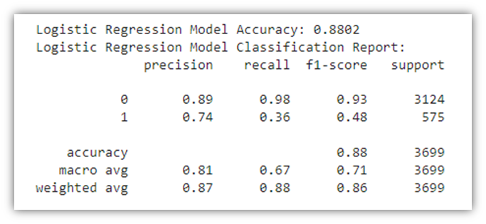
The results of both the confusion matrix and the table report show that the model accuracy is 88%, which is great in this case. The results also highlight the high model accuracy when predicting true negatives (98%), which would mean that the model excels in predicting when the user session does not end in a purchase. However, the precision for class1 (false negatives), is relatively lower, signifying that the model will correctly predict whether or not a user session will end in a purchase 74% of the time. To look at prediction test results from another perspective, an ROC curve can be informative:
					# Plot ROC curve for Logistic Regression
svc_disp = RocCurveDisplay.from_estimator(log_reg, X_test_scaled, y_test,
                                          name="Logistic Regression", color="darkorange")

plt.title('ROC Curve for Logistic Regression')
plt.show()
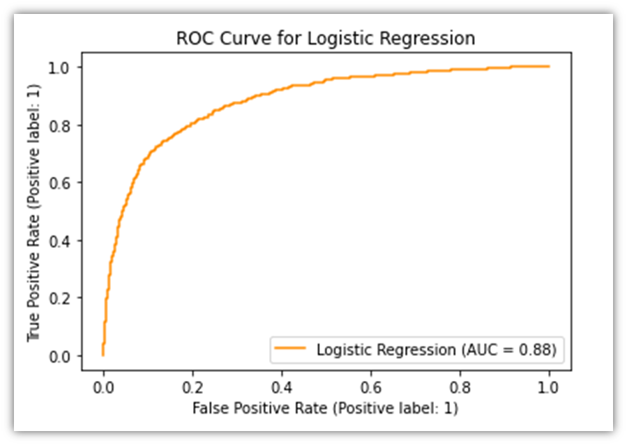
The ROC Curve allows the viewer to visually evaluate the performance of predictive model. It plots the percentage of two of the four measures in the confusion matrix, namely the True Positive and the False Positive. The orange line signifies how accurately the model performs. If the line was diagonal, it would mean that the predictions made by the model were random. However, since the line is arched upwards, it means that there are more instances of True Positives than can be derived from random chance.
Another powerful tool for predicting user purchases is Random Forest, which is a robust predictive model that internally employs several predictive models resulting in high accuracy results (Tan et al., 2019). Because it can examine a wide range of information from our data this approach is effective in improving predictions by combining multiple decision trees. It assists us in determining the factors that influence a customers decision to purchase. Furthermore it excels at avoiding errors caused by assuming that something operates in one way when in reality it operates in another. Because of this we can see how users might behave on the website with great benefit from Random Forest. Similar to the way Logistic Regression was implemented, here’s how to utilize it:
					df3 = pd.get_dummies(df)
X = df3.drop(['Revenue_True', 'Revenue_False'], axis=1)
y = df['Revenue'].astype(int)  # Ensuring 'Revenue' is numeric

# Split the dataset into training and testing sets
X_train, X_test, y_train, y_test = train_test_split(X, y, test_size=0.3, random_state=42)

# Standardizing the features (important for Logistic Regression)
scaler = StandardScaler()
X_train_scaled = scaler.fit_transform(X_train)
X_test_scaled = scaler.transform(X_test)


# Random Forest Classifier
rf_clf = RandomForestClassifier(n_estimators=100, random_state=42)
rf_clf.fit(X_train, y_train)  # No need to scale features for Random Forest

# Predictions
rf_predictions = rf_clf.predict(X_test)
Nearly the same steps in Logistic Regression were taken to apply Random Forest Classifier. The only difference is that with Random Forest, the features do not need to be scaled, so no scaling function was used.
As we did before, let’s test how this prediction model performs:
					# Random Forest Confusion Matrix
rf_cm = confusion_matrix(y_test, rf_predictions)
sns.heatmap(rf_cm, annot=True, fmt='d', cmap='Purples')
plt.title('Random Forest Confusion Matrix')
plt.xlabel('Predicted')
plt.ylabel('True')
plt.show()
					# Random Forest Model Accuracy
rf_accuracy = accuracy_score(y_test, rf_predictions)
print(f"Random Forest Model Accuracy: {rf_accuracy:.4f}")

# Random Forest Model Report
print("\nRandom Forest Model Classification Report:")
print(classification_report(y_test, rf_predictions))
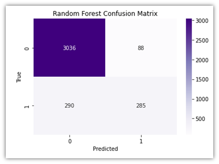
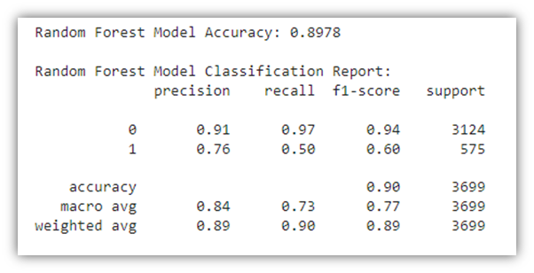
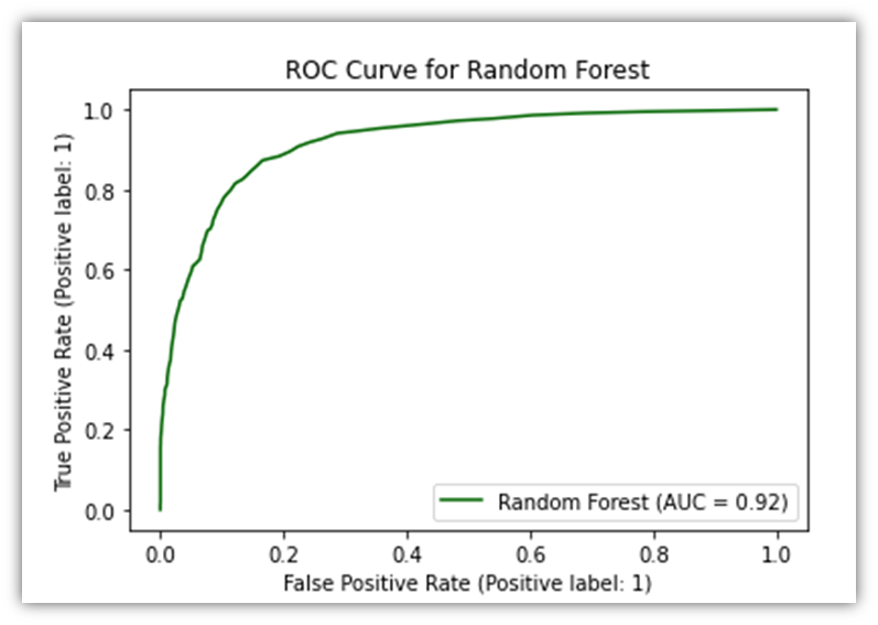
The results of the Random Forest Classifier prediction module closely resemble those of the Logistic Regression previously discussed. The same interoperations also apply here. Let’s generate the ROC curve here as well:
					# Now use X_test_scaled_df with RocCurveDisplay.from_estimator
RocCurveDisplay.from_estimator(rf_clf, X_test, y_test,
                               name="Random Forest", color="darkgreen")
plt.title('ROC Curve for Random Forest')
plt.show()
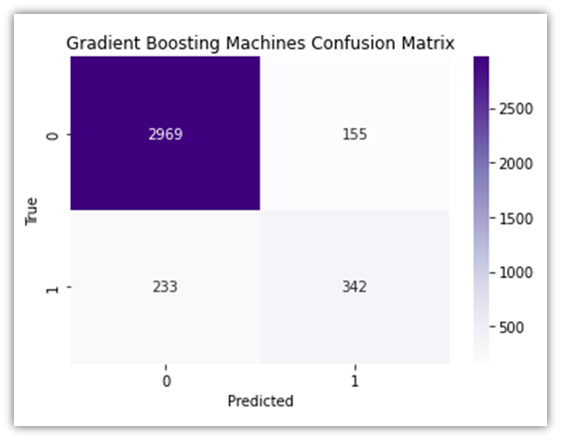
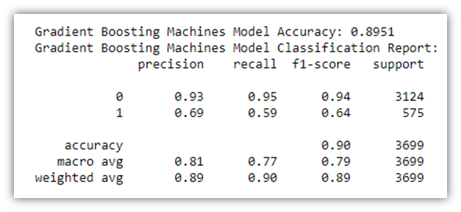
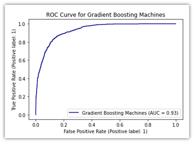
Another predictive analysis tool we could use is GBM. Because of its sophisticated methodology we use Gradient Boosting Machines (GBM) in our analysis to forecast customer purchase behavior on GlobalGoods. Due to its high effectiveness for our dataset complexity GBM sequentially corrects errors from a series of decision trees to improve prediction accuracy. This approach is excellent at breaking down complex data patterns and quickly pinpointing important variables affecting purchase decisions (Kuhn and Johnson, 2013). The ability of GBM to process various kinds of data and to fine-tune the model makes it a powerful model in our toolbox that offers valuable insights into customer interactions on the e-commerce platform. Implementation of this tool is almost identical to the Random Forest Classification. Therefore, to avoid repetition, the visuals will be put here without the associated code:
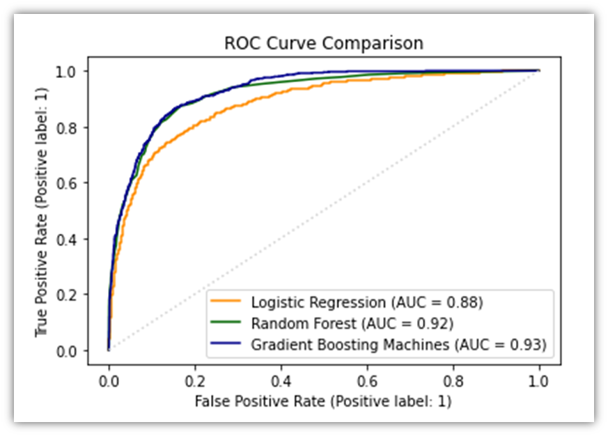
Now let’s combine all three ROC curves for the sake of comparison.
					# Start a new matplotlib figure
plt.figure(figsize=(10, 8))

# Plot ROC curve for Logistic Regression
RocCurveDisplay.from_estimator(log_reg, X_test_scaled, y_test, name="Logistic Regression", color="darkorange")

# Plot ROC curve for Random Forest on the same figure
# Make sure that X_test is appropriately preprocessed if needed to match the training conditions of rf_clf
RocCurveDisplay.from_estimator(rf_clf, X_test, y_test, name="Random Forest", color="darkgreen", ax=plt.gca())

RocCurveDisplay.from_estimator(gbm_clf, X_test, y_test, name="Gradient Boosting Machines", color="darkblue", ax=plt.gca())


# Adding plot title and adjusting layout
plt.title('ROC Curve Comparison')
plt.plot([0, 1], [0, 1], color='lightgrey', linestyle=':')  # Diagonal line for reference
plt.show()
After we’re done training the model and testing it, we may download the resulting dataset:
log_reg_result_df = pd.DataFrame(log_reg_predictions)
Model Deployment
Our investigation into the factors that influence a customer’s decision to purchase from GlobalGoods revealed that the website’s functionality depends heavily on the use of models such as Logistic Regression. This model has the ability to quickly determine whether a customer will make a purchase based on their behavior on the website. Customers are therefore more likely to purchase when this estimate is used to present them with exclusive offers or goods they might find appealing. What makes a customer likely to buy is revealed by the thorough examination we conducted using Random Forest and GBM models. This implies that depending on what the models tell us we can use marketing to send emails or display advertisements that are more likely to pique the interest of the consumer. This improves our marketing since it speaks directly to the preferences of the consumer. Additionally we can facilitate customers purchases by using these models. We can make that section of our website easier if we observe that customers stop purchasing after a particular amount of time. Perhaps as a result fewer people will walk away empty-handed. We also discussed adjusting prices according to our estimation of what a customer will be willing to pay. In addition to helping us sell more by ensuring that the price is exactly right for each customer this must be done carefully to maintain the customers’ trust. We must continuously feed our models new data about customer behavior if we hope to improve them. This implies that the models predictions will improve with time. To make GlobalGoods better for customers we need to use the insights from the models which means that everyone from computer experts to ad makers needs to collaborate in order to do this well.
Limitations of The Different Prediction Models
In this study we examined various approaches to forecast customer purchase intent using models such as Random Forest Gradient Boosting Machines (GBM) and Logistic Regression. There are certain situations in which each of these approaches might not be the most effective for the type of data we have. The logic behind Logistic Regression is very simple to comprehend. However it may miss all the nuanced ways in which various aspects of the customers’ behavours and actions interact to influence their purchasing decisions. The relationships in this model are best described as linear but purchasing goods can involve more. One major benefit of Random Forest is that it allows us to examine much more intricate relationships within our data. However it requires a lot of processing power and time to run particularly when we employ a large number of trees to improve our predictions. Additionally if there is a lot of random noise in our data this model may become overly fixated on insignificant details mistakenly believing they hold greater significance than they actually do. Because GBM builds trees one at a time each of which aims to correct mistakes from the previous one it represents a further advancement in the pursuit of incredibly accurate predictions. However it takes a lot of adjusting its settings to get it just right and this can take some time to figure out. Like Random Forest it can also begin to interpret the noise in our data as significant patterns if were not careful which could result in predictions that dont always pan out. We learned from looking at these models that it is impossible to predict with 100% accuracy whether a customer will make a purchase. Every approach has advantages and disadvantages of its own particularly when attempting to apply it to the vast array of data that exists in e-commerce such as that found at GlobalGoods. It serves as a reminder that in order to better understand our customers we should never stop experimenting and may even need to combine several approaches to achieve the greatest outcomes.
Discussion and Analysis Conclusion
As we come to the end of the discussion and analysis section of our study we are left to consider a journey that went beyond the simple use of predictive models such. We have learned a great deal about the huge potential that lies within data analysis thanks to this insightful journey through the challenging landscape of consumer behavior on the GlobalGoods e-commerce platform. We witnessed firsthand how important a comprehensive and varied analytical approach is in unlocking the layers of consumer decision-making processes by closely observing how customers use the platform. The section has covered a wide range of topics including data preparation analysis and the complex field of predictive modeling.
Conclusion and Recommendations
To sum up our report, we looked into determining the factors that influence consumers decisions to buy products on the e-commerce platform known as GlobalGoods. Our work started with meticulous data preparation, and following that we analyzed the data in-depth to look for trends and areas of interest, and lastly we applied predictive models like Random Forest and Logistic Regression to forecast consumer behavior, namely, whether or not a customer will buy a product in the site given the customer session details. Putting together the pieces of a large puzzle was the analogy for each step. Our research journey has demonstrated to us how fascinating and intricate it is to comprehend why consumers choose to make an online purchase. To determine which approaches could provide us with more insight into the behavior of our customers we employed a variety of techniques. For instance while Random Forest covered more ground and produced a more robust prediction, Logistic Regression was simpler to comprehend and provided us with more precise insights. However our job is not over yet. We still have a great deal of work ahead of us. We can use the ever-improving technology and data analysis techniques to increase the accuracy of our predictions. Additionally we should work to learn more about how to tailor each customers shopping experience as this may boost the possibility that they will make a purchase. It’s essential that businesses such as GlobalGoods make decisions based on data at all times. Better marketing strategies and website functionality can be achieved by understanding customers preferences and behavior. In this manner customers may find what they’re looking for more quickly and may be more inclined to make a purchase. Working on this project was ultimately a fantastic learning opportunity. The e-commerce industry is evidently highly dynamic and anticipating customer behavior is incredibly valuable. There is still much to be discovered and refined as the actions we have taken in this article are only the beginning. In order for businesses to prosper in a competitive online marketplace the objective is to keep improving at comprehending and forecasting the behavior of customers. Developing a story that encapsulates the fundamentals of e-commerce dynamics has been more important than merely testing models. The knowledge gained here is a starting point for further research and a more comprehensive comprehension of how digital consumer interactions can be used to create more stimulating and profitable e-commerce environments. As we look ahead its clear that there are plenty of opportunities for additional research and development in the field of data analytics in e-commerce. The information we have assembled here represents only a small portion of what is feasible. With a variety of analytical tools and techniques at our disposal were ready to delve even further in the future to improve our forecasts and tactics. This project which is based on the thorough analysis that was done paves the way for upcoming efforts that will improve the online shopping experience increase conversion rates and provide a competitive advantage in the crowded market.
References
Aggarwal, C.C. and Reddy, C.K. (eds) (2014) Data clustering: algorithms and applications. Boca Raton: CRC Press (Chapman & Hall/CRC data mining and knowledge discovery series).
C. Sakar, Y.K. (2018) ‘Online Shoppers Purchasing Intention Dataset’. [object Object]. Available at: https://doi.org/10.24432/C5F88Q.
Hastie, T., Tibshirani, R. and Friedman, J.H. (2017) The elements of statistical learning: data mining, inference, and prediction. Second edition, corrected at 12th printing 2017. New York, NY: Springer (Springer series in statistics). Available at: https://doi.org/10.1007/b94608.
Kuhn, M. and Johnson, K. (2013) Applied predictive modeling. New York: Springer.
Tan, P.-N. et al. (2019) Introduction to data mining. Second edition. New York: Pearson.
Witten, I.H. et al. (2017) Data mining: practical machine learning tools and techniques. Fourth edition. Amsterdam Boston Heidelberg London New York Oxford Paris San Diego San Francisco Singapore Sydney Tokyo: Elsevier, Morgan Kaufmann.